Zero Delay Feedback Filters, Part II

IMPROVING OUR ONE POLE LOW PASS

In his book, Vadim Zavalishin points out that the equation that this structure implements,

can be re-written as

Then we can say that

 and

Which makes our overall equation look like this:

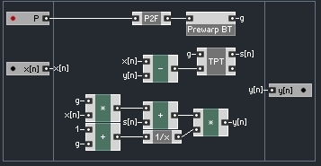
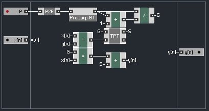
This is a very easy modification to make:

Not only does this save us a bit of CPU by not multiplying by 1/(1+g) every sample (unless we actually need to), but it also makes the math coming up substantially easier. Notice that since all incoming values to the integrator are scaled by G, and s[n] is dependant upon these values, there is no further modification needed to convert s[n] to S.

MS-20 FILTER

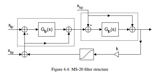
Some time ago, I stumbled across the following diagram of the signal flow of an MS-20 filter:

The original paper can be found here. The little blocks that say Glp(s) are one pole low pass filters (we can use the filter we just designed to fulfill this role). There is a shaper in the feedback loop that will be dropped for now for simplicity’s sake. The triangle with a ‘k’ next to it is an amplifier (multiply operation) that controls the resonance, or feedback.

I have not attempted to build a high pass or band pass version of this filter yet, so we will focus on the low pass (IE, using the Xlp input).

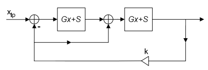
Dropping the shaper, and high pass and bandpass outputs, our structure looks like this:

Just like we did with the one pole filter, let’s begin by trying to find an equation that describes the value of the output, which I will again refer to as y[n].

The output of the first Glp(s) block can be written as:

to which the value of k*y is immediately added. This makes the input to our second low pass equal to:

meaning the output of the second low pass (and the filter as a whole) is:

S1 is the S value of the first one pole low pass, and S2 is the S value of the second. Both filters use the same G value. Once again, we must solve for y. We can begin by multiplying using the distributive property:

Now, rearrange so that all values of y are one the same side of the equation like so:

Now, factor out y:

Finally, divide both sides by (1+G^2k-Gk)

To build a structure that realizes this equation in Reaktor, it makes sense to extend our one pole low pass to also output it’s S value. Once we do this, the macro must have it’s ‘Solid’ parameter unselected in properties.

Finally, our new structure will have two one pole structures, and each will use the same G value, so it makes sense to calculate G outside of the macro. Our new one pole macro looks like this:

Let’s build a simple structure to follow the diagram of the MS-20 filter:

k is given to have a value between 0 and 2 in the text.

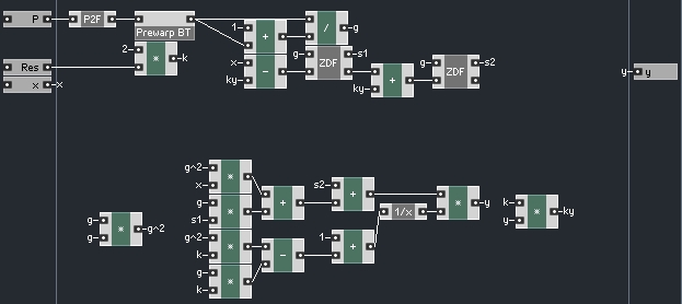
Now all that is left is to calculate y  using the formula we calculated above, and use that value to calculate ky:

This leaves us with an MS-20 structure that has a substantially improved behaviour over the traditional method, in several respects: improved frequency response (IE the cutoff point is where it belongs), improved resonant behaviour (the resonance stays constant in amplitude across the structure, and better frequency range (the original filter will only accept a cutoff range between 50Hz and 10kHz).
Here’s the structure of the original filter, made using the bilinear transform:

One interesting thing I noticed when comparing the two is that they are identical with the resonance (k) turned all the way down (other than the improved cutoff range of the zero delay version). This makes perfect sense, since the behavior we have been modifying is the feedback.

CONCLUSION

I have included a sample ensemble that is a modification of the EzFFT Filter Analyzer. This ensemble contains the two MS-20 macros, and graphs them in the same area with different colors. This way you can easily compare two filters. I found this tool to be invaluable in my work for this tutorial.

Download here.

The Lin/Log switch determines whether the graph is linear or logarithmic. Log is the suggested setting, but there are times when I find a linear graph to be useful. The ensemble also includes a bandlimited sawtooth oscillator. You can use the switch to choose between the zero delay feedback (ZDF) and traditional (BiLin) filters to be applied to the sawtooth. This allows for simple A/B comparison.

The topic of zero delay feedback is pretty complicated but once you grasp it the math for simpler designs like these is not so complicated. If there are any questions, please feel free to ask in the comments.